Maximizing Penguin Classification Accuracy with Minimal Features
Author
Anweshan Adhikari
Introduction to the Data Set
The Palmer’s Penguin dataset collected by Dr. Kristen Gorman and the Palmer Station, Antarctica LTER, includes physical measurements of individuals from three different penguin species: Chinstram, Gentoo and Adelie. Some of the features in included culmen length, culmen depth, mass body, flipper length and so on. In this blog posts, we will try to find a group of three features that will achieve maximum accuracy for linear regression, K-nearest Neighbour Classifier, Random Forest Classifier and decision tree classifiers.
Before we get into finding the features, let’s start by exploring our dataset. The table shown below shows the glimpse of our data.
Code
import pandas as pdtrain_url ="https://raw.githubusercontent.com/middlebury-csci-0451/CSCI-0451/main/data/palmer-penguins/train.csv"train = pd.read_csv(train_url)train.head()
studyName
Sample Number
Species
Region
Island
Stage
Individual ID
Clutch Completion
Date Egg
Culmen Length (mm)
Culmen Depth (mm)
Flipper Length (mm)
Body Mass (g)
Sex
Delta 15 N (o/oo)
Delta 13 C (o/oo)
Comments
0
PAL0708
27
Gentoo penguin (Pygoscelis papua)
Anvers
Biscoe
Adult, 1 Egg Stage
N46A1
Yes
11/29/07
44.5
14.3
216.0
4100.0
NaN
7.96621
-25.69327
NaN
1
PAL0708
22
Gentoo penguin (Pygoscelis papua)
Anvers
Biscoe
Adult, 1 Egg Stage
N41A2
Yes
11/27/07
45.1
14.5
215.0
5000.0
FEMALE
7.63220
-25.46569
NaN
2
PAL0910
124
Adelie Penguin (Pygoscelis adeliae)
Anvers
Torgersen
Adult, 1 Egg Stage
N67A2
Yes
11/16/09
41.4
18.5
202.0
3875.0
MALE
9.59462
-25.42621
NaN
3
PAL0910
146
Adelie Penguin (Pygoscelis adeliae)
Anvers
Dream
Adult, 1 Egg Stage
N82A2
Yes
11/16/09
39.0
18.7
185.0
3650.0
MALE
9.22033
-26.03442
NaN
4
PAL0708
24
Chinstrap penguin (Pygoscelis antarctica)
Anvers
Dream
Adult, 1 Egg Stage
N85A2
No
11/28/07
50.6
19.4
193.0
3800.0
MALE
9.28153
-24.97134
NaN
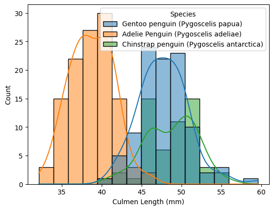
Continuing the exploration, the graph below shows the distribution of Culmen Lengths for each penguin species
Code
import seaborn as snsimport matplotlib.pyplot as plt# Plot the distribution of Culmen Lengths for each penguin speciessns.histplot(data=train, x="Culmen Length (mm)", hue="Species", kde=True, bins=15)
The histogram plot shows the distribution of culmen length for three different Penguins’ species: Adelie, Chinstrap, and Gentoo. The x-axis represents the culmen length values, and the y-axis represents the count of penguins falling into each bin, where each bin size is specified to 15. From the plot, we can see that Gentoo and Chinstrap penguins have a similar distribution of culmen length, with a peak around 45-50 mm, while Gentoo penguins have smaller culmen length, ranging from around 30mm-46mm with a peak around 40 mm. The histogram also shows the shape of the data distribution for each penguin species, with overlaid smooth curves that represent the density estimate. This helps to identify any overlapping areas or differences in the tails of the distributions. Based on the culmen lengths, it would be possible to distinguish between Adelie Penguins from the other two species with a high accuracy. However, the accuracy would be minimal in distinguishing between Chinstrap Penguin and Gentoo Penguin based on their culmen range, as both species have similar culmen lengths.
Similarly, the table offers a convenient way to compare the physical attributes of the penguin species.
Code
penguin_stats = train.groupby("Species").aggregate({"Body Mass (g)": "mean", "Flipper Length (mm)": "mean"}) #Finiding the mean of body mass and flipper length for each species.penguin_stats = penguin_stats.round(0) # Rounding the values to zero decimal placepenguin_stats.columns = ["Avg. Body Mass (g)", "Avg. Flipper Length (mm)"] # Renaming the columns print(penguin_stats)
Based on the average measurements, the Adelie penguins have a smaller body mass and shorter flipper length compared to the other species. In contrast, the Gentoo penguins have the largest values for both of these features. The Chinstrap penguin, however, falls somewhere in the middle of the other two species. The table can serve as reference values to determine the species of an individual penguin based on their physical characteristics. For example, if a penguin has a body mass and flipper length that are close to the average measurements for a particular species, it is likely that the penguin belongs to that species.
Data Cleaning and Preparation
Below, the Palmer’s penguin dataset is being prepared to serve as the training set for the machine learning models. The code drops irrelevant columns in the dataset, removes rows with missing values, converts target variable, species, into numbers and scales the quantitative features.
Code
import itertoolsfrom sklearn.preprocessing import LabelEncoder, StandardScalerfrom sklearn.model_selection import cross_val_scorefrom sklearn.tree import DecisionTreeClassifierfrom sklearn.neighbors import KNeighborsClassifierfrom sklearn.linear_model import LogisticRegressionimport warningswarnings.filterwarnings("ignore")le = LabelEncoder()le.fit(train["Species"])def prepare_data(df):# Drop irrelevant columns df = df.drop(["studyName", "Sample Number", "Individual ID", "Date Egg", "Comments", "Region"], axis=1)# Remove rows with missing values and unknown sex df = df[df["Sex"] !="."] df = df.dropna()# Encode the target variable y = le.transform(df["Species"]) df = df.drop(["Species"], axis=1)# One-hot encode categorical features df = pd.get_dummies(df)# Scale the quantitative features scaler = StandardScaler() quant_cols = ['Culmen Length (mm)', 'Culmen Depth (mm)', 'Flipper Length (mm)', 'Body Mass (g)', 'Delta 15 N (o/oo)', 'Delta 13 C (o/oo)'] df[quant_cols] = scaler.fit_transform(df[quant_cols])return df, yX_train, y_train = prepare_data(train)
Code
import warningsfrom itertools import combinationsfrom sklearn.ensemble import RandomForestClassifierwarnings.filterwarnings("ignore")all_qual_cols = ['Island', 'Clutch Completion', 'Sex']all_quant_cols = ['Culmen Length (mm)', 'Culmen Depth (mm)', 'Flipper Length (mm)', 'Body Mass (g)', 'Delta 15 N (o/oo)', 'Delta 13 C (o/oo)']best_score_LR =0best_score_KNN=0best_score_RF =0best_score_DT =0for qual in all_qual_cols: qual_cols = [col for col in X_train.columns if qual in col]for pair in combinations(all_quant_cols, 2): cols =list(pair) + qual_cols# Training on Logistic Regression LR = LogisticRegression() LR.fit(X_train[cols], y_train) lr_score = LR.score(X_train[cols], y_train)# Updating the best score and columns for Logistic Regressionif lr_score > best_score_LR: best_cols_LR = cols best_score_LR = lr_score best_LR = LR# Training on K-nearest Neighbour Classifier KNN = KNeighborsClassifier() KNN.fit(X_train[cols], y_train) knn_score = KNN.score(X_train[cols], y_train)# Updating the best score and columns for k-Nearest Neighbors Classifierif knn_score > best_score_KNN: best_cols_KNN = cols best_score_KNN = knn_score best_KNN = KNN# Training on Random Forest Classifier RF = RandomForestClassifier(max_depth=3, random_state=0) RF.fit(X_train[cols], y_train) rf_score = RF.score(X_train[cols], y_train)# Updating the best score and columns for Random Forest Classifierif rf_score > best_score_RF: best_cols_RF = cols best_score_RF = rf_score best_RF = RF# Training on Decision Tree Classifier DT = DecisionTreeClassifier(max_depth=3) DT.fit(X_train[cols], y_train) dt_score = DT.score(X_train[cols], y_train)# Updating the best score and columns for Decision Tree Classifierif dt_score > best_score_DT: best_cols_DT = cols best_score_DT = dt_score best_DT = DTprint("Best 3 columns for LR: "+str(best_cols_LR))print("Best 3 columns for KNN: "+str(best_cols_KNN))print("Best 3 columns for RF: "+str(best_cols_RF))print("Best 3 columns for DT: "+str(best_cols_DT))
Best 3 columns for LR: ['Culmen Length (mm)', 'Culmen Depth (mm)', 'Island_Biscoe', 'Island_Dream', 'Island_Torgersen']
Best 3 columns for KNN: ['Culmen Length (mm)', 'Culmen Depth (mm)', 'Sex_FEMALE', 'Sex_MALE']
Best 3 columns for RF: ['Culmen Length (mm)', 'Culmen Depth (mm)', 'Island_Biscoe', 'Island_Dream', 'Island_Torgersen']
Best 3 columns for DT: ['Culmen Length (mm)', 'Culmen Depth (mm)', 'Island_Biscoe', 'Island_Dream', 'Island_Torgersen']
In this section, I used four Sckit learn’s machine learning models- logistic regression, k-nearest neighbor, random forest, and decision tree classifiers- to find the 3 combination of features that resulted in the highest accuracy scores. The accuracy of each combination of three features was then compared to find the combination that resulted in the highest accuracy score.
Code
# Prepare the test datatest_url ="https://raw.githubusercontent.com/middlebury-csci-0451/CSCI-0451/main/data/palmer-penguins/test.csv"test = pd.read_csv(test_url)X_test, y_test = prepare_data(test)# Evaluate the performance of each model on the test datatest_score_LR = best_LR.score(X_test[best_cols_LR], y_test)test_score_KNN = best_KNN.score(X_test[best_cols_KNN], y_test)test_score_RF = best_RF.score(X_test[best_cols_RF], y_test)test_score_DT = best_DT.score(X_test[best_cols_DT], y_test)# Print the test scoresprint("Test score for LR: "+str(test_score_LR))print("Test score for KNN: "+str(test_score_KNN))print("Test score for RF: "+str(test_score_RF))print("Test score for DT: "+str(test_score_DT))
Test score for LR: 0.9852941176470589
Test score for KNN: 0.9705882352941176
Test score for RF: 0.9705882352941176
Test score for DT: 0.9852941176470589
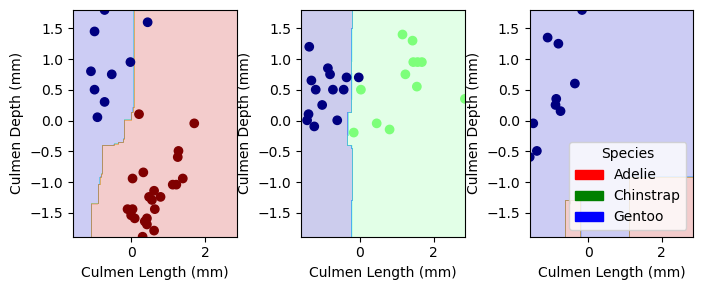
Our trained models were not able to achieve a 100% accuracy score in the test data. However, we identify that Logistic regression and decision tree yeild the best accuracy scored on classifying penguins. MOving forwards we will consider both Logistic regression and decision tree to be the best model for classifying penguins
Code
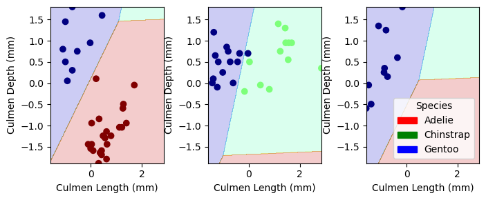
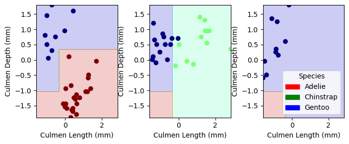
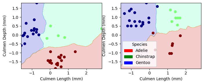
from matplotlib.patches import Patchimport matplotlib.pyplot as pltimport numpy as npdef plot_regions(model, X, y): x0 = X[X.columns[0]] x1 = X[X.columns[1]] qual_features = X.columns[2:] fig, axarr = plt.subplots(1, len(qual_features), figsize = (7, 3))# create a grid grid_x = np.linspace(x0.min(),x0.max(),501) grid_y = np.linspace(x1.min(),x1.max(),501) xx, yy = np.meshgrid(grid_x, grid_y) XX = xx.ravel() YY = yy.ravel()for i inrange(len(qual_features)): XY = pd.DataFrame({ X.columns[0] : XX, X.columns[1] : YY })for j in qual_features: XY[j] =0 XY[qual_features[i]] =1 p = model.predict(XY) p = p.reshape(xx.shape)# use contour plot to visualize the predictions axarr[i].contourf(xx, yy, p, cmap ="jet", alpha =0.2, vmin =0, vmax =2) ix = X[qual_features[i]] ==1# plot the data axarr[i].scatter(x0[ix], x1[ix], c = y[ix], cmap ="jet", vmin =0, vmax =2) axarr[i].set(xlabel = X.columns[0], ylabel = X.columns[1]) patches = []for color, spec inzip(["red", "green", "blue"], ["Adelie", "Chinstrap", "Gentoo"]): patches.append(Patch(color = color, label = spec)) plt.legend(title ="Species", handles = patches, loc ="best") plt.tight_layout()